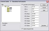
ATS SPC shows the control limits for all the features in a batch in the Control Limits dialog. The tree view on the left allows you to choose a feature to examine and the right hand side shows the current control limit values.
Control limits form the main weapon of SPC in distinguishing special cause variation from common cause variation. They are calculated statistically from your measured data and represent the range of variation you would expect to see in the manufacturing process producing any given feature of your parts. If the parts that you measure fall outside these control limits the process is exhibiting variation above and beyond what is expected of it. In other words – something has gone wrong!
ATS SPC shows the control limits for all the features in a batch in the Control Limits dialog. The tree view on the left allows you to choose a feature to examine and the right hand side shows the current control limit values. |
|
You must have a batch open in Data Entry mode…
1. From the SPC menu, choose Control Limits.
The Control Limits dialog opens, showing you a list of features and the limits, if any, currently used in the highlighted feature.
2. In the left hand pane of the dialog window, click on a feature or press the Up and Down cursor keys to choose a feature.
The right hand side of the Control Limits dialog shows the limits currently used in the selected feature.
3. Click the Done button to close the Control Limits dialog.
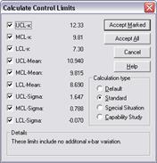
The Calculate Control Limits dialog shows the new values of control limits calculated from the current measured data. There are four methods of calculating limits, detailed formulae for each method, if required, can be found below. |
|
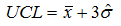
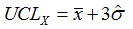
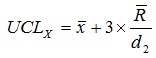
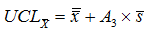
The general rule of thumb with control limits is to calculate points at 3 standard deviations either side of the mean. Hence…
 and
and 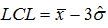
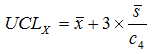
In practice, for largely historical reasons, the mean sigma or mean
range from the chart is used, along with a number of empirically derived
table factors, to calculate an estimate of standard deviation,  , or 'sigma-hat'.
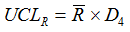
Standard Limits
Standard limits are calculated from the mean and the average range or sigma of the measured data according to motor industry standard formulae.
 and
and 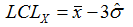
Using the standard table factors these become, in a mean/sigma feature…
 and
and 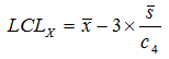
…and in a mean/range feature…
 and
and 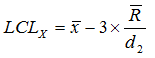
The limits for the means are given by…
 and
and 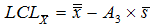
or
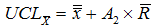 and
and 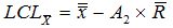
And the limits for sigmas…
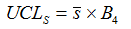 and
and 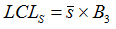
and ranges…
 and
and 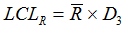
If the feature has an additional mean variation value, VADD, this has the effect of widening the mean and individual limits by the amount of additional variation.
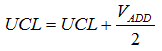 and
and 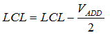
Limits for spreads, i.e. sigmas or ranges, are not affected by VADD
The Additional Mean Variation is entered in the SPC Parameters dialog: choose Parameters from the SPC menu. See Additional Mean Variation for details.
Default Limits
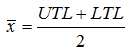
The default limits are not calculated from data but from the feature’s tolerance limits. By assuming individual control limits equal to the tolerance limits ATS SPC back-calculates a value for standard deviation and from that calculates appropriate limits for the mean and the sigma or range.
 and
and 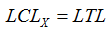
Mean and Standard deviation are estimated from tolerances…
 and
and 
Standard deviation is used, along with the table factors c4 or d2, to calculate values for mean sigma and mean range…
 and
and 
…and then the standard limits formulae can be used as given above.
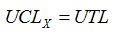
Special Situation Limits
This method is used when the limits for the mean chart can’t be calculated using the mean sigma or range. Instead ATS SPC calculates mean limits from the grand mean and the standard deviation of the subgroup means. The sigma or range limits are calculated in the same way as standard limits.
NB Special Situation Control Limits are not implemented in this version of ATS SPC
Capability Study Limits
This method derives control limits from the results of the last capability study performed on the feature. The limits for individuals are equal to the performance limits and thus account for the distribution shape, while those for the mean and sigma or range charts are calculated using the standard deviation from the capability study.
 and
and 
The mean and standard deviation from the study are used to calculate values for mean sigma or mean range and these are used in the standard limits formulae as above.
You must have a batch open in Data Entry mode.
 If
you need to enter an additional mean variation you should do so before
calculating the control limits. See Additional Mean Variation
for details on page 85.
If
you need to enter an additional mean variation you should do so before
calculating the control limits. See Additional Mean Variation
for details on page 85.
1. From the SPC Menu, choose Control Limits.
Using the mouse…
2. In the Control Limits dialog select a feature to calculate by clicking on the required feature in the left hand pane.
3. Click the Calculate button to open the Calculation dialog.
4. Click the radio button for the type of limits you want to calculate: Default, Standard, Special Situation or Capability Study.
ATS SPC shows the new limit values before you apply them.
5. Click the Accept All button to use the new limit values or check the limits you want to use, clear those you don’t want and then click the Accept Marked button to use just the marked limits and leave the others unchanged.
6. Back in the Control Limits dialog repeat the above for any further features or click the Done button to close.
Using the keyboard…
2. In the Control Limits dialog select a feature to calculate by pressing the Up and Down keys to highlight a feature name on the left.
3. Press [Alt+C] to open the Calculation dialog.
4. Choose the type of limits to calculate by pressing [Alt+D] for Default limits, [Alt+S] for Standard, [Alt+P] for Special Situation, or [Alt+C] for Capability Study limits.
ATS SPC shows the new limit values before you apply them.
5. Press [Alt+A] to use all the new limits or press Tab to move the focus to the limit check boxes and then Space to check or clear the limits. Then press [Alt+M] to use only the marked limits and leave the others unchanged.
6. Back in the Control Limits dialog repeat the above for any further features or press Tab to highlight the Done button and then Enter to close.
In most processes which produce a normally distributed output there is a relationship between the variation found in the mean chart and that in the spread chart. A process with wide spread control limits will also have wide mean control limits. Some processes however produce a very small part to part variation but, over a longer time scale, show a wider than expected variation in the mean chart. A grinding process, for example, drifts as the grinding wheel wears but then shifts back again when the wheel is dressed or replaced. A drilling process will exhibit sudden shifts as drill bits are changed, since the drill bits themselves vary from one to the next.
Such processes would normally show out of control points due to middle third failure in the spread chart or to drifts or runs in the mean chart. They can be accommodated by adding a small additional variation to the mean chart only. In the case of the drill bits this would be the expected spread of drill bit sizes. In the grinding process is would be the allowable deterioration of the wheel before redressing. ATS SPC adds half of this variation to the upper mean (and individuals) control limit and subtracts half from the lower limits. The spread limits are not changed at all.
Select a feature in the tree view at the top of the dialog box. Then, in the edit box at the bottom, type in the required variation to be added into the mean and individuals control limits for that feature. Click OK or press ENTER to save the value.
There is a checkbox in the Control Limits dialog determining whether or not newly calculated control limits should be applied back over previous data in the batch. If you check this box in the course of calculating new control limits ATS SPC will apply the new limits to all the data in the batch. If you don’t check the box the new limits will apply only from this point onwards.
Typically you will project the limits back only when determining control limits for the first time for a new process. The idea is to calculate limits from only data that is in control – in other words to achieve self-consistent limits calculated only from in-control data. This ensures that special cause variation is excluded from the control limit calculation. You should collect around 20-25 subgroups of data and then calculate control limits – using the Standard Limits formula. Project the new limits back and check that everything is in control. If not then eliminate the out of control subgroups and recalculate the limits. Repeat this until all the remaining data in control within the limits calculated from it.
From this point on you should work to these limits and whenever the process strays out of control you should investigate the cause and eliminate any affected subgroups. Over a period of time you will probably find that , not only do you find and eliminate the special cause variations but patterns will be become apparent in some of the remaining, variation and you will be able to investigate and eliminate variation previously thought to be ‘common causes’, i.e. inherent in the process. As this happens you will be able to recalculate the control limits – moving them inwards to account for removal of variation. In these cases you would typically not project the limits back over old data but would preserve the old limits so that the chart becomes a record of the process improvement.
Note that you cannot project control limits back if you are using a signed database to meet traceability requirements.
ATS SPC detects chart points beyond the control limits and warns you what has happened in the Subgroup Out Of Control window (‘OOC window’). This appears at the end of the subgroup containing the out of control condition and details exactly what has gone wrong.
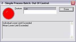
The OOC window shows the batch and feature name, or names, and a list of the conditions ATS SPC has detected – there may be more than one.
If the batch contains more than one out of control feature then all are listed and you can examine the problems in each feature by selecting it from the feature list box (press the Down key or click the feature you want to examine).
The conditions listed are those which ATS SPC has been configured to report in the ‘subgroup’ column of the control reporting switches. See Control Switches for details of how to configure what constitutes an out of control condition.
As well as simple control limit violations ATS SPC also looks for trends in the chart data and can report these as OOC conditions too. See Trends for more details.
As well as simple control limit violations ATS SPC also looks for trends in the chart data and can report these as OOC conditions too.
ATS SPC can detect the following trends in both the mean and the spread (sigma or range) chart…
Drifts
A ‘drift’ is a sequence of continuously increasing or continuously decreasing chart points. Seven points all progressively bigger than the previous point is, statistically, about as likely as throwing 7 heads in a row and is therefore a significant indicator of a change in the process that should be investigated.
Runs
A ‘run’ is a sequence of chart points all to one side of the chart mean, all above or all below. Like drifts, a run of 7 or more points is unlikely and is sufficient reason to investigate the cause.
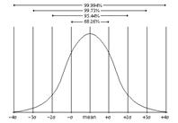
Middle Third
The middle third rule is a quick test for normally distributed data. Roughly two thirds (actually 68%) of the data from a normal distribution falls into the middle one third of the distribution. The remaining one third of the data falls into the two outer thirds of the distribution. (see picture). |
|
ATS SPC assumes that the control limits represent the spread of the chart data and reports if significantly more or less than two thirds of the chart points fall into the middle third of the region between the control limits. Note that this test is often turned off for the spread chart since ranges in particular typically do not follow the normal distribution.